# Libraries
library(tmap)
library(sf)
library(terra)
library(raster)
library(stars)
library(ggplot2)
library(plotly)
library(dplyr)
library(ggspatial)
library(patchwork)Background Information
In February 2021, Texas suffered a major power power crisis with more than 4.5 million homes and businesses were left without power for several days1. Historically power outages have disproportionately affected people of color and low income communities. They take longer to recover from the disaster because of fewer resources available to them2. More information regarding the engineering and political background are hyper linked.
I am interested in investigating if socioeconomic status played a factor in community recovery from the power outage.
Data
My analysis utilized the following data sets:
Visible Infrared Imaging Radiometer Suite
Remotely-sensed night light raster I am interested in tiles from 2021-02-07 and 2021-02-16.
This contains - Subset of roads that intersect the Houston metropolitan area - Houses in the Houston Metropolitan area
U.S. Census Bureau’s American Community Survey (ACS)
Contains socioeconomic data for each census block
Data Preparation
Load Libraries
Load the necessary libraries. I will mainly be working with stars, sf and ggplot2.
Night Lights
First import all of the required data using the stars package. Then it can be conjoined into a single composite.
## Import tiles for 2021-02-07 and 2021-02-16
# tile h08v05, collected on 2021-02-07
feb7_h <- read_stars("data/VNP46A1/VNP46A1.A2021038.h08v05.001.2021039064328.tif")

# tile h08v06, collected on 2021-02-07
feb7_v <-read_stars("data/VNP46A1/VNP46A1.A2021038.h08v06.001.2021039064329.tif")

# tile h08v05, collected on 2021-02-16
feb16_h <- read_stars("data/VNP46A1/VNP46A1.A2021047.h08v05.001.2021048091106.tif")

# tile h08v06, collected on 2021-02-16
feb16_v <- read_stars("data/VNP46A1/VNP46A1.A2021047.h08v06.001.2021048091105.tif")

## Convert to stars object
stars_207 <- st_mosaic(feb7_h,feb7_v)
stars_216 <- st_mosaic(feb16_h,feb16_v)
I am interested in seeing the difference in night lights intensity from before and after the storm.
# change in night lights intensity (2/07 - 2/16)
change_lights <- stars_207 - stars_216
I assume that any location that experienced a drop of more than 200 NW cm-2sr-1 experienced a blackout. Locations that experienced a drop of less than 200 NW cm-2sr-1 did not experience a blackout and are assigned NA values.
# reclassify differences: blackout (> 200 nWcm^-2^sr^-1) and NA (<200)
dem_rcl <- cut(change_lights,
              breaks=c(-Inf,200,Inf),
              labels = c("blackout","no blackout"))

# assign `NA` to all locations that experienced a drop of *less* than 200 nW cm^-2^sr^-1
change_lights[change_lights <= 200] = NA
My area of interest is the Houston metropolitan area and is located within the following coordinates: (-96.5, 29), (-96.5, 30.5), (-94.5, 30.5), (-94.5, 29). I can crop my blackout mask to this area.
# Define the Houston metropolitan area
coord_box <- matrix(c(-96.5,29,-96.5,30.5,-94.5,30.5,-94.5,29,-96.5,29),
                    ncol = 2,
                    byrow = TRUE)

# Create a polygon with coordinates
polygon <- st_polygon(list(coord_box))

# Convert the polygon into a simple feature collection
# Assign the CRS to blackout lights tiles
polygon_sf <- st_sfc(polygon, crs = st_crs(blackout_mask))

# Crop (spatially subset) the blackout mask to our region of interest
houston_mask <- st_crop(blackout_mask,polygon_sf)

# Reproject cropped blackout dataset to EPSG:3083
houston_mask <- st_transform(houston_mask, crs = "EPSG:3083")
Highways
Highways typically account for most of the night light seen from space. To remove the potential error of identifying the wrong areas, I will exclude highways from the blackout mask.
The roads geopackage contains more than highway data so using SQL I selected just motorway data.
Once I have selected the necessary data I can buffer and identify areas that experience blackouts further than 200m from a highway.
# Re-project data to EPSG:3083
highway <- st_transform(highway,crs = "EPSG:3083")

# Identify areas within 200m of all highways
highways_200 <- highway %>% st_buffer(dist = 200) %>%  st_union()

## Identify the areas in houston that experienced blackouts further than 200m from a highway
houston_blackout <- st_difference(houston_mask,highways_200)
Homes Impacted by Blackout
Using SQL I selected only residential buildings from OpenStreetMap. Residential buildings include: residential, apartments, house, static caravan, and detached.
#SQL query to select only residential buildings
query <- "SELECT * FROM gis_osm_buildings_a_free_1 WHERE (type IS NULL AND name IS NULL) OR type in ('residential', 'apartments', 'house', 'static_caravan', 'detached')"

# Import residential buildings
buildings_data <- st_read("data/gis_osm_buildings_a_free_1.gpkg", query = query)

# Transform buildings data CRS to EPSG:3083
buildings_data <- st_transform(buildings_data, crs = "EPSG:3083")
I can now filter to count the number of homes impacted within the blackout areas.
# Filter to homes within blackout areas
homes_blackout <- buildings_data %>% st_filter(houston_blackout,
                          .predicate = st_intersects)

paste("Number of impacted homes:",nrow(homes_blackout))
[1] "Number of impacted homes: 157410"Socioeconomic Factors
The ACS data is composed of geodatabase layers. The geometries are stored in the ACS_2019_5YR_TRACT_48_TEXAS layer and income is stored in the median income field B19013e1. Using SQL both of these can be filtered to.
#View ACS layers
st_layers("data/ACS_2019_5YR_TRACT_48_TEXAS.gdb")
# Read in geometries and change CRS to EPSG 3083
texas_geometries <- st_read("data/ACS_2019_5YR_TRACT_48_TEXAS.gdb",
                          layer = "ACS_2019_5YR_TRACT_48_TEXAS") %>%
  st_transform(crs = "EPSG:3083")

# Read in ACS data in X19_INCOME layer and select B19013e1 column
texas_median_income <-
  st_read("data/ACS_2019_5YR_TRACT_48_TEXAS.gdb",
    layer = "X19_INCOME") %>%
  select('GEOID', 'B19013e1') %>%
  rename("median_income" = 'B19013e1',
         "GEOID_Data" = "GEOID")
I am only interested in income census tracts that experienced blackouts in the Houston boundaries. Through spatial joining and cropping I can filter to these specific census blocks.
# Join the income data to the census tract geometries
income_geom <- left_join(texas_geometries,texas_median_income, by = "GEOID_Data") %>% st_transform(crs = "EPSG:3083")

# Transform Houston polygon CRS to match income_geom
polygon_sf <- st_transform(polygon_sf, crs = st_crs(income_geom))

# Crop census income data to just Houston area
houston_geom <- st_crop(income_geom,polygon_sf)

## spatially join census tract data with buildings determined to be impacted by blackouts
houston_blackout <- st_join(houston_geom,homes_blackout, left = FALSE)

## Census tracts had blackouts - by unique census track
paste("Number of unique census tracks had blackouts:",length(unique(houston_blackout$GEOID)))
[1] "Number of unique census tracks had blackouts: 754"Visualization
I can visualize a map of median income by census tract, designating which tracts had blackouts by outlining them.
#Create a map of median income by census tract
# Census tracts that had blackouts are designated as red
visual <- ggplot() +
  geom_sf(data = houston_geom, aes(fill = median_income)) +
  geom_sf(
    data = houston_blackout,
    aes(color = 'red'),
    fill = NA,
    show.legend = 'abs'
  ) +
  scale_fill_viridis_c() +
  scale_color_identity(guide = "legend",name = "",labels = "Blackout area", breaks = 'red') +
  annotation_scale(location = 'bl', width = 0.1) +
  annotation_north_arrow(location = 'br',height = unit(.8, "cm"),
  width = unit(.8, "cm"), style = north_arrow_fancy_orienteering()) +
  labs(title = "Houston Median Income Across Census Tracks with Blackouts") +
  theme_minimal()

visual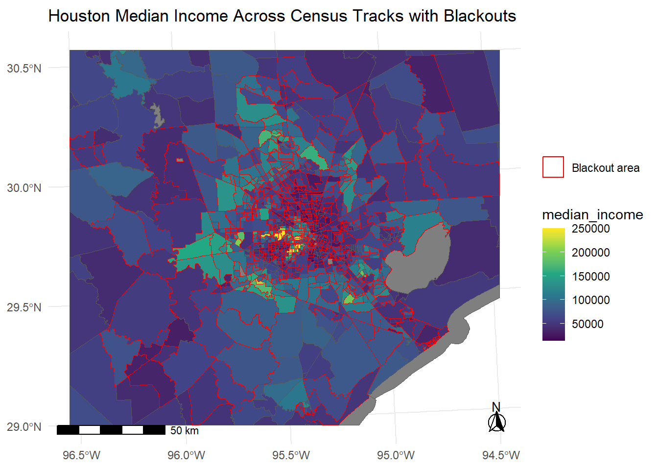
To get a better understanding of the distribution of income in impacted and un-impacted zones, I plotted them as histograms side-by-side.
# Simplify and clean Houston census tracks in blackout zone
houston_blackout_dist <- houston_blackout %>%
  select(GEOID,median_income) %>% unique()

# Income distribution on impacted census tracts
p1 <- ggplot(houston_blackout_dist, aes(x = median_income)) +
  geom_histogram(bins = 20, fill = 'orange', color = 'black') +
  labs(x = 'Median Income', y ='Count', title = 'Income Distribution of Impacted Census Tracts') + ylim(0,150) + theme(text=element_text(size=7))

#Clean up Houston geom
houston_geom_dist <- houston_geom %>% select(GEOID,median_income) %>% unique

# Identify the census track that were not affected by the blackout
houston_non <- setdiff(houston_geom_dist,houston_blackout_dist)

# Plot income distribution of census tracts not affected by the blackout
p2 <- ggplot(data = houston_non, aes(x = median_income)) +
  geom_histogram(bins = 20,
                 fill = '#4398F9',
                 color = 'black') +
  ylim(0, 150) +
  labs(x = "Median Income",
       y = "Count",
       title = "Income Distribution of Unimpacted Census Tracts") +
  theme(text = element_text(size = 7))

# Turn plots interactive
p1 <- ggplotly(p1)

p2 <- ggplotly(p2)

# Set them side by side
subplot(p1, p2, nrows = 1)
Conclusion
The income distribution of the impacted census tract has a similar distribution of the un-impacted census tract. They both display a right skew with the majority of the distribution being in the lower income range. During this storm income level of the census tract did not display a large effect based solely on the graphs generated. There are some limitations to this study such as the limitation of spatial data in the days during the storm because of the cloud coverage. The raster data I analyzed is during the second storm and does not account for the third storm. Also, there is the issue of the year the ACS data represents. The income demographic are from 2019, these could have changed since then and potentially do not accurately represent the income distribution of Houston during the storm.
Footnotes
Douglas, E. (2021, February 20). Gov. Greg Abbott wants power companies to “Winterize.” Texas’ track record won’t make that easy. The Texas Tribune. https://www.texastribune.org/2021/02/20/texas-power-grid-winterize/↩︎
Dobbins, J., & Tabuchi, H. (2021, February 16). Texas blackouts hit minority neighborhoods especially hard. Texas Blackouts Hit Minority Neighborhoods Especially Hard. https://www.nytimes.com/2021/02/16/climate/texas-blackout-storm-minorities.html↩︎
Citation
BibTeX citation:
@online{vaquero,
  author = {Vaquero, Hazel},
  title = {Houston 2021 {Power} {Outage:} {Socioeconomic} {Analysis}},
  url = {https://hazelvaq.github.io/blog/2023-12-13-houston-power-outage/},
  langid = {en}
}
For attribution, please cite this work as:
Vaquero, Hazel. n.d. “Houston 2021 Power Outage: Socioeconomic
Analysis.” https://hazelvaq.github.io/blog/2023-12-13-houston-power-outage/.